Aligning Housing with Climate Goals: The Importance of Measuring VMT

Authors:
Rachel Strangeway, Assistant Specialist
Zack Subin, Associate Research Director

Download the PDF with additional maps and resources

Introduction

California has undertaken two challenging housing and climate goals: to build 2.5 million new homes by 2030 and to reduce climate pollution 40 percent by 2030.^[1] Especially given that passenger travel represents the single largest source of climate pollution from California households, geographically defined transportation criteria are increasingly being used in California housing policy to promote state goals for reducing climate pollution (Appendix Table 2). These goals target reductions in the amount of daily driving by California residents, as measured in a metric known as vehicle miles traveled (VMT) per person.^[2]

Previous Terner Center commentaries have investigated the mechanisms by which, and to what extent, building more housing in walkable neighborhoods could reduce VMT by enabling future residents to drive less while accomplishing their daily activities. In general, research suggests infill housing—building new housing within existing neighborhoods—tends to reduce carbon pollution by avoiding more carbon-intensive development in new suburban neighborhoods.

Following Senate Bill (SB) 226 (2011), the Office of Land Use and Climate Innovation (LCI—formerly the Office of Planning and Research) developed statutory guidance defining “low vehicle travel areas” (i.e., neighborhoods with relatively low VMT per person). In addition, LCI developed technical guidance expanding on this definition for the implementation of SB 743 (2013). Both documents offer criteria for streamlined impact assessment under the California Environmental Quality Act (CEQA),^[3] meaning that housing development in these areas may proceed somewhat more quickly, or at less expense, through local environmental review.

LCI defined low-VMT neighborhoods by comparing neighborhood-level VMT patterns to a regional or city average. LCI’s reasoning was that new housing development in low-VMT neighborhoods would enable future residents to also drive less. California State Governor Gavin Newsom’s August 2024 executive order encouraging infill housing recommended the use of LCI’s Site Check tool, a web-based mapping platform launched by LCI in 2023, to identify opportunities for streamlined development, including low-VMT neighborhoods under LCI’s definition.

All of this suggests that how “low-VMT” is defined, as well as the data and models that are used to measure local VMT patterns, are increasingly important to where new housing is incentivized. Methodological changes can alter which neighborhoods are defined as low-VMT, thereby influencing which developments may be provided streamlined CEQA entitlement processes.

In this analysis, we compare the low-VMT layer from LCI’s Site Check tool (a composite of state and regional models described below: “the State’s low-VMT layer”) with two other modelled approaches to measuring VMT, to note differences in which neighborhoods are identified as having low-VMT under different approaches.

We find large differences in the low-VMT maps depending on which VMT model is used, as well as whether neighborhood-level VMT is compared with a regional or state VMT baseline.

Importantly, the State’s low-VMT layer may be overlooking many higher-resource and job-rich neighborhoods that have the potential to reduce VMT and support the state’s fair housing goals when building new housing.^[4] We recommend that the State further invest in developing and validating VMT models for use in housing policy, and consider expanding the criteria for defining low-VMT to include larger areas for streamlining housing development.

Existing VMT models

VMT per person for a certain geographic area can be measured in two different ways: based on total driving occurring within the area, or on total driving done by people living within the area. For example, you could measure the VMT in San Francisco using the miles driven within the city limits, including incoming commuters for the portions of their trips occurring within the city’s boundary. Or, you could measure the VMT based on how much San Francisco residents drive in a typical day, including their miles driven outside the city’s boundaries. The first metric is more common and easier to measure since it can be observed directly by counting vehicles using highways and major roadways. This approach is how the Federal Highway Administration (FHWA) reports VMT for each county. However, the second metric (“residential VMT”) is more relevant for housing policy, since it accounts for whether people are able to live close to their work and/or easily access other daily needs such as grocery stores or schools. Residential VMT is used under the LCI guidance, as well as in the models assessed below.

LCI’s Site Check tool is designed to help developers identify sites that could qualify a development for CEQA exemption or streamlining (above), including VMT criteria, as well as other policy criteria such as minimizing exposure to environmental hazards. The Site Check tool compiles VMT estimates from regional or state agencies and identifies areas in which VMT is below the regional average and 15 percent below the regional average at a traffic analysis zone (TAZ) level.^[5] These VMT estimates are not actual measurements of residential travel, but rather composites of model outputs from either regional Metropolitan Planning Organization (MPO) VMT models or the California Statewide Travel Demand Model (CSTDM), depending on the region (Appendix 3).

To understand the implications of using alternative VMT estimates for housing policy, we compare the areas contained in the State’s low-VMT layer to those similarly defined using two other models: Replica and Local Area Transportation Characteristics for Households Data (LATCH). Replica is a private company that uses a proprietary model calibrated using data from mobile devices, such as cell phone locations, to estimate U.S. travel patterns. LATCH is a federal model incorporating 2017 National Household Travel Survey (NHTS) data and American Community Survey (ACS) data. Previous research has compared LATCH and Replica, finding modest evidence that Replica’s estimates are realistic and appropriate for housing policy analysis.^[6] In this analysis, we map neighborhoods with an average VMT 15 percent below each model’s respective regional averages.

We also attempt to validate the VMT models in Site Check, Replica, and LATCH with two additional sets of VMT estimates: those from FHWA and from Fehr and Peers’ VMT+ model (model details can be found in Appendix 3). Neither of these can be compared directly at a neighborhood scale with the three VMT models;^[7] instead, we compare regional- and state-average VMT estimates.

It is important to note that in all three of these model layers (the State’s low-VMT layer, Replica, and LATCH), the actual miles travelled are not directly observed (e.g., from vehicle count data, trip diaries, or household travel surveys), but are instead modeled estimates of resident trips and aggregated VMT. These tools rely on modelling because of the lack of fine geographic-scale, residential VMT datasets; collecting this type of data would be very challenging.^[8] However, each model also comes with its own underlying assumptions and limitations, which is why understanding differences in how they designate low-VMT areas is important.

Findings

Effects of VMT Model Selection

Our analysis shows that the choice of model influences which neighborhoods are designated as low-VMT, with implications for where new housing would be streamlined. In coastal urban areas, more neighborhoods are designated low-VMT according to Replica than using either the State’s low-VMT layer or LATCH, while in less dense inland cities there are more neighborhoods designated low-VMT according to the State than using Replica (Figures 1 and 2; Appendix Tables A8 and A9).

Figure 1: Map of the South Bay comparing Replica low-VMT areas (blue) to the State’s low-VMT layer (red)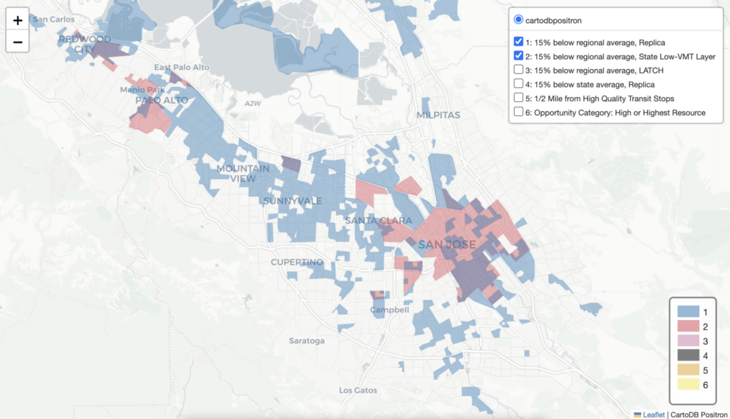There are more low-VMT areas in the South Bay with Replica (shown in blue) than with the State’s low-VMT layer (shown in red).

Figure 2: Map of San Bernardino comparing Replica low-VMT areas (blue) to the State’s low-VMT layer (red)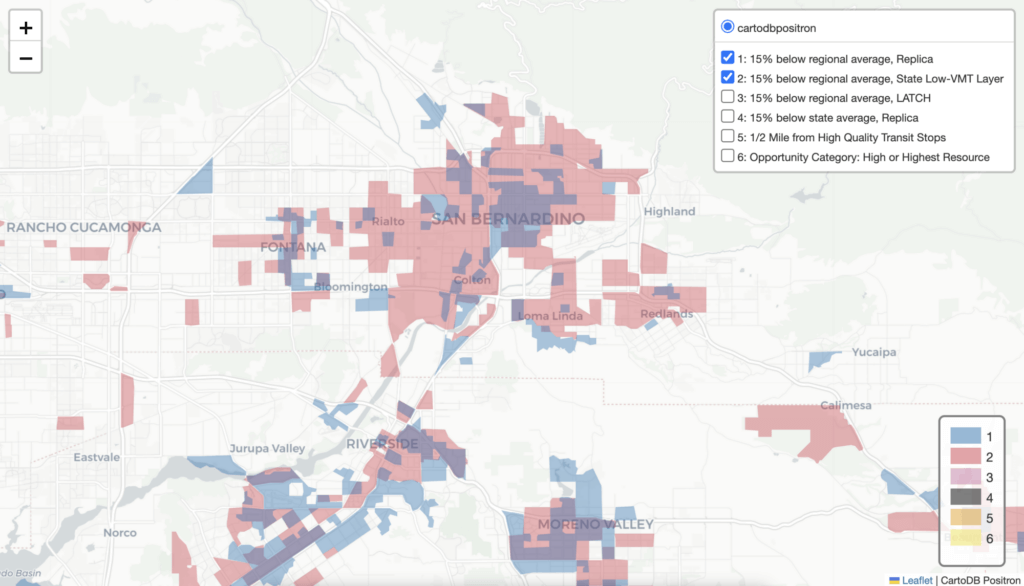There are more low-VMT areas in San Bernardino with the State’s low-VMT layer (shown in red) than with Replica (shown in blue).

For example, Replica designates 62 percent of Los Angeles’ city population as living in low-VMT neighborhoods, while the State designates 40 percent. Overall, Replica designates 1.9 times as many Los Angeles County residents’ neighborhoods as low-VMT as the State does. In contrast, the State designates about 71 percent of San Bernardino’s city population as living in low-VMT neighborhoods, while Replica designates 29 percent; overall, Replica designates half as much of San Bernardino County as low-VMT as the State does.

We find that the State’s low-VMT layer identifies fewer coastal urban neighborhoods and more inland city neighborhoods for streamlined housing development than if Replica’s model were used.

Building more in coastal urban areas would help reduce carbon pollution and provide access to job-rich urban centers. However, development in inland areas may provide new housing at lower cost. The State’s housing plan envisions all regions of the state contributing to overall housing production, so developing more infill housing in both areas would be ideal.

Effects of VMT Baseline Definition

Additionally, we find that the identification of low-VMT neighborhoods is sensitive to the baseline used, with implications for different regions of the state.

For example, the Bay Area region has a relatively low average VMT compared to the statewide average in all three models (as well as both of the additional data sources used for validation; Table 1). According to Replica’s modeling, people in several neighborhoods next to downtown Mountain View average 17 VMT per person, per day^[9]—more than 15 percent less than Replica’s state average of 21 but not its regional average of 19 VMT per person, per day.

If low-VMT neighborhoods were defined relative to the state average, about 40 percent more residents’ neighborhoods in the Bay Area would be identified for housing development streamlining (Appendix Figure A6; Table A8). Since the goal is to reduce statewide carbon pollution, using the state, rather than the regional, average as the baseline would lead to overall greater reductions in VMT.^[10]

In contrast, using a statewide baseline would yield fewer neighborhoods for streamlining in higher-VMT regions of the state, such as the Central Valley. Using a statewide baseline may also require changing LCI’s statutory guidance implementing SB 226. In these cases, it could make sense to use the existing regional, rather than state, baseline.

Relationship with Transit Proximity

LCI guidance suggests streamlining for locations within a half mile of “high-quality transit” under SB 743.^[11] We compare these locations to neighborhoods designated in the State’s low-VMT layer and Replica. In coastal cities, the State tends to designate fewer neighborhoods low-VMT, so most of these would already be covered by the high-quality transit definition (Appendix Figure A4). In Replica, however, including low-VMT neighborhoods expands streamlining modestly in coastal cities (Appendix Figure A3). Inland, the State designates many neighborhoods low-VMT but not within a half mile of high-quality transit (Appendix Figure A5).

Overall, the expansion of eligibility for CEQA streamlining from transit-proximate to also include low-VMT may modestly expand the areas streamlined, but for different locations in the State’s low-VMT layer and Replica.

Relationship with Opportunity Maps

Neighborhoods that are low-VMT (which tend to be in more dense, urban areas) may differ from those that have better schools and other resources to support economic mobility (which tend to be wealthier, single-family suburbs). To explore this relationship, we overlay the low-VMT models with the higher-resourced neighborhoods defined by the state’s 2024 Opportunity Maps.^[12] We find that using Replica instead of the State’s low-VMT layer (or LATCH) would enhance overlap between low-VMT areas and higher-resource areas (Figure 3, Figure 4).

Figure 3: Map of the San Jose area comparing the State’s low-VMT layer (red) to higher-resource areas (yellow)
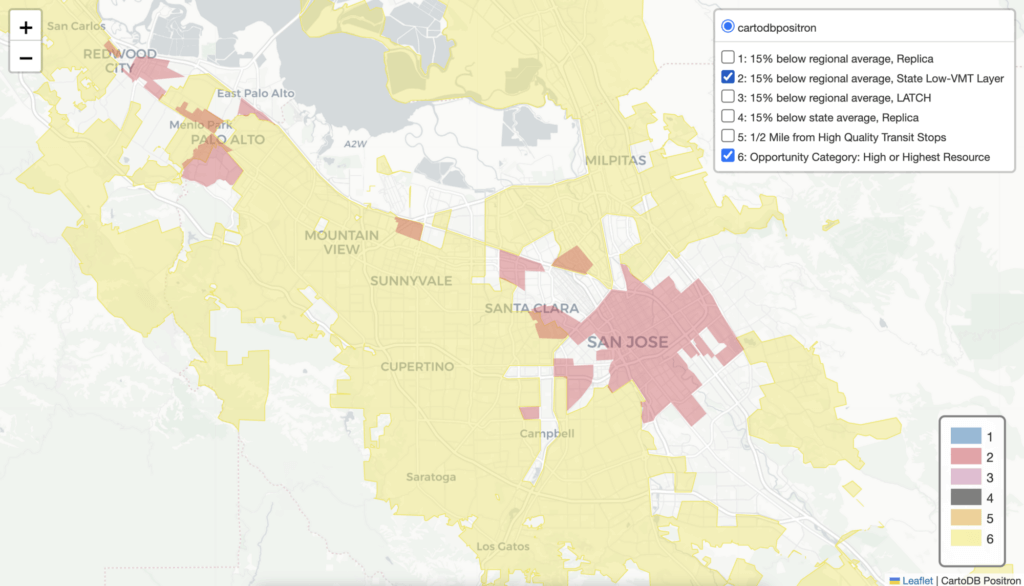There is very little overlap between higher-resource areas and the State’s low-VMT layer.

Figure 4: Map of the San Jose area comparing Replica low-VMT areas (blue) to higher-resource areas (yellow)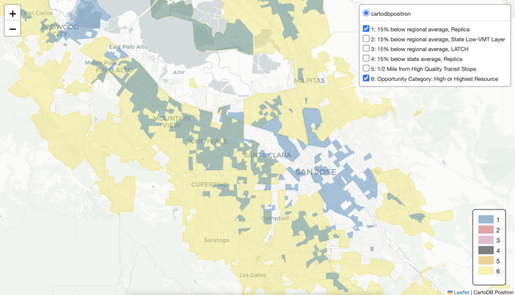There is more overlap between higher-resource areas and low-VMT areas from Replica.

The choice of VMT model would affect how much area is identified as satisfying both environmental and fair housing criteria for housing development.

Interactive Statewide Map of Transportation and Housing Policy Criteria

This interactive map illustrates how low-VMT neighborhoods may vary depending on the model estimates used across the state. The map also illustrates High-Quality Transit Areas^[13] and higher-resource areas (i.e., “high” or “highest” resource areas) defined in the state’s 2024 Opportunity Map.

Policy Implications

Given the urgency of both addressing climate change and the state’s housing shortage, this analysis suggests that policymakers should pay more attention to how “low-VMT” areas are defined. We recommend that the State allocate additional research and technical assistance funds to make high-quality, transparent, and comprehensive VMT estimates available to the public.^[14] Given the challenges of validating VMT models (Appendix 1), the State may first commission detailed expert review of the various existing approaches to measuring VMT (including acquiring proprietary datasets). Then, technical assistance funding could be used to either: (1) support regional transportation planning agencies, prioritizing lower-resourced regions, to improve and harmonize their models; or (2) to enhance the validation and transparency of the California State Travel Demand Model to promote consistency of VMT modelling across the state.

In the face of imperfect measurements of residential VMT, policymakers could also develop broader transportation criteria to expand where new housing is streamlined or otherwise encouraged. For example, they could enable streamlining for neighborhoods that are either designated low-VMT or have characteristics associated with lower VMT such as high residential density and high walkability scores: enabling housing projects located in neighborhoods satisfying any of these three criteria.

Given the State’s climate goals, policymakers should consider revising guidance to use the statewide VMT average as the baseline in regions with low average VMT, rather than using their regional average as the baseline. To avoid reducing housing production in regions with higher average VMT, policymakers may continue to use the existing baseline there. Using different baselines in different regions of the state may help balance state greenhouse gas reduction and housing production goals.

The use of VMT estimates to guide planning and policy decisions is important for building a sustainable California. However, policymakers should avoid letting imperfect information obscure opportunities for much-needed housing development. Considering the holistic environmental benefits of infill and/or dense housing beyond reducing VMT, they should err on the side of streamlining more existing neighborhoods for new housing.

Appendix 1: Validation of VMT Estimates

To contextualize the differing low-VMT areas identified by each model, we compared the regional average VMT per person inferred in each model with each other and with FHWA estimates (Table 1). FHWA regional estimates for VMT, based on measuring total driving occurring in an area (above), are uncorrelated with any of the three VMT model layers measuring driving by residents in an area (the State’s low-VMT layer, Replica, and LATCH)—illustrating the difference between the two approaches. However, while Replica estimates are statistically similar to those of LATCH, the State’s composite estimates are not correlated with any of the other models’.^[15]

While the results of measuring VMT based on miles driven in an area versus the miles driven by residents of an area differ greatly at the local level, they become more similar when focusing on larger geographic areas, as their included trips overlap more. For example, commuters frequently cross city lines but rarely cross state lines, especially in a large state like California.

Comparing the statewide averages for all five models, LATCH estimates appear to be systematically lower then FHWA estimates, while Replica and the State’s estimates match more closely on average,^[16] within the margin expected from year-to-year variation and differences in model scope.^[17]

The statewide averages mask larger regional differences between the State’s low-VMT layer and the other models: the State’s VMT estimates are lower than those of other models for MPOs with small populations (Table 1). For example, the State’s low-VMT layer estimates Madera County’s average to be 10.0 VMT per person per day, lower than the other models for any region. We attempted to understand the differences between the State’s low-VMT layer and the other estimates more closely, but the downloadable layer does not provide sufficient information to enable direct, quantitative validation and cross-comparison; key missing information includes VMT estimates covering the entire state (not just areas designated low-VMT) and geographic metadata for the transportation analysis zones.^[18]

Table 1: Regional Average of Daily Vehicle Miles Traveled Per Capita according to State (2019-2021), Replica (2023), LATCH (2017), VMT+ (2024),^[19] and FHWA (2022).

MPO (Year Represented)	State (2019- 2021)	Replica (2023)	LATCH (2017)	VMT+ (2019)	FHWA (2022)	Population (ACS five-year estimates, 2022)
AMBAG	15.7	22.9	13.5	22.8	22.2	770,933
BCAG	14.9	22.5	14.4	22.3	19.8	213,605
FCOG	16.1	21.3	12.0	20.9	22.4	1,008,280
KCAG	18.1	24.6	13.0	23.1	29.2	152,515
KCOG	17.1	21.6	12.5	22.4	28.0	906,883
MCAG	17.6	20.7	12.4	25.7	27.9	282,290
MCTC	10.0	27.6	12.1	27.4	31.6	157,243
MTC	15.5	18.9	14.1	19.4	19.4	7,685,888
SACOG	20.8	21.1	14.0	23.1	21.3	2,537,783
SANDAG	19.0	21.9	13.6	21.2	21.9	3,289,701
SBCAG	11.5	21.1	13.2	19.3	20.5	445,213
SCAG	20.8	20.6	12.4	20.6	21.6	18,743,554
SJCOG	19.5	21.8	12.5	26.6	23.2	779,445
SLOCOG	15.4	25.8	16.2	22.9	30.3	281,712
SRTA	18.8	26.2	15.2	22.3	27.9	181,852
StanCOG	17.5	20.5	12.7	24.2	22.0	552,063
TCAG	15.1	20.4	12.4	22.7	23.3	473,446
TMPO	19.0	35.4	15.7		14.7	55,771
Statewide totals[20]	18.9	20.7	13.0	21.0	21.6	38,518,177

 

References

Bureau of Transportation Studies. (2024). Methodology for 2017 Local Area Transportation Characteristics for Households. Bureau of Transportation Statistics. https://www.bts.gov/latch/latch-methodology-2017

California Environmental Quality Act (CEQA) Appendix M: Performance Standards for Infill Projects Eligible for Streamlined Review, Public Resources Code Sections 21094.5 and 21094.5.5. (2016). California Governor’s Office of Land Use and Climate Innovation. https://resources.ca.gov/CNRALegacyFiles/ceqa/docs/2016_
CEQA_Statutes_and_Guidelines_Appendix_M.pdf

California Governor’s Office of Planning and Research (OPR). (2018). Technical Advisory: On Evaluating Transportation Impacts in CEQA. https://lci.ca.gov/docs/20190122-743_Technical_Advisory.pdf

California Tax Credit Allocation Committee (CTCAC). (2024). Methodology for Opportunity and High-Poverty & Segregated Area Mapping Tools. https://www.treasurer.ca.gov/ctcac/opportunity/2024/draft-2024-opportunity-mapping-methodology.pdf

CTCAC, & California Department of Housing and Community Development (HCD). (2024). Final 2024 CTCAC HCD Opportunity Map [Dataset]. https://belonging.berkeley.edu/final-2024-ctcac-hcd-opportunity-map

Environmental Protection Agency (EPA). (2025). National Walkability Index [Dataset]. https://epa.maps.arcgis.com/home/item.html?id=f16f5e2f84884b93b380cfd4be9f0bba

Federal Highway Administration (FHWA). (2025). Highway Statistics Series: Annual Vehicle Distance Traveled in Miles and Related Data by Highway Category and Vehicle Type (VM–1; Version 2022) [Dataset]. Highway Statistics Series. https://www.fhwa.dot.gov/policyinformation/statistics/2022/vm1.cfm

Fehr & Peers. (n.d.). SB 743 Policy Adoption Technical Assistance Program: Establishing an Infill and Affordable Housing Screen (VMT Policy Adoption Technical Assistance Memo Template). Association of Bay Area Governments. Retrieved March 14, 2025, from https://abag.ca.gov/sites/default/files/documents/2024-04/MTC_Infill_Housing_VMT_White_Paper.pdf

Heyerdahl, J., & Conservation Biology Institute. (2023a). 15% Below Regional Average Vehicle Miles Traveled (VMT) Per Capita, California (Version 2.1) [Dataset]. Data Basin. https://databasin.org/datasets/4e189c878e094cbfb0a000ae8ad04948/

Heyerdahl, J., & Conservation Biology Institute. (2023b). Below Regional Average Vehicle Miles Traveled (VMT) Per Capita, California (Version 2.1) [Dataset]. Data Basin. https://databasin.org/datasets/d155d4bec8774c7db030ab090bd86359/

Jones, C., & Kammen, D. M. (2014). Spatial distribution of U.S. household carbon footprints reveals suburbanization undermines greenhouse gas benefits of urban population density. Environmental Science and Technology, 48(2), 895–902. https://doi.org/10.1021/es4034364

Kim, J. H., et. al. (2024). Assessing the Potential for Densification and VMT Reduction in Areas Without Rail Transit Access. https://doi.org/10.7922/G22V2DGJ

Little Hoover Commission. (2024). CEQA: Targeted Reforms for California’s Core Environmental Law (279). https://lhc.ca.gov/wp-content/uploads/Report279.pdf

Manville, M. (2024). Induced Travel Estimation Revisited. UCLA Institute for Transportation Studies. https://escholarship.org/uc/item/8m98c8j1

Marantz, N. J., et. al. (2024). Evaluating the Potential for Housing Development in Transportation-Efficient and Healthy, High-Opportunity Areas in California (20STC009; pp. 1–178). California Air Resources Board. https://www.law.virginia.edu/node/2182176

Miller, E. (2023). The current state of activity-based travel demand modelling and some possible next steps. Transport Reviews, 43(4), 565–570. https://doi.org/10.1080/01441647.2023.2198458

Office of Governor of California Gavin Newsom. Executive Order N-2-24 (2024). https://www.gov.ca.gov/wp-content/uploads/2024/07/infill-EO.pdf

Othering and Belonging Institute (OBI). (2024, January 18). California renews adoption of OBI opportunity map | Othering & Belonging Institute, University of California, Berkeley. https://belonging.berkeley.edu/california-renews-adoption-obi-opportunity-map

Reid, C., Subin, Zack, & McCall, J. (2024). Housing + Climate Policy: Building Equitable Pathways to Sustainability and Affordability. Terner Center for Housing Innovation, University of California, Berkeley. https://ternercenter.berkeley.edu/research-and-policy/climate-housing-overview/

Replica. (2024, January). Seasonal Mobility Model Methodology Extended (Places). Replica. https://documentation.replicahq.com/docs/seasonal-mobility-model-methodology-extended-places

Subin, Z. (2024, October 9). How much can new housing contribute to state climate action? Terner Center for Housing Innovation, UC Berkeley. https://ternercenter.berkeley.edu/blog/how-much-can-new-housing-contribute-to-state-climate-action/

Subin, Z. (2024, March 12). Understanding the Role of New Housing in Reducing Climate Pollution. Terner Center for Housing Innovation, UC Berkeley. https://ternercenter.berkeley.edu/research-and-policy/role-of-new-housing-in-reducing-climate-pollution/

Subin, Z., et. al. (2024). US urban land-use reform: A strategy for energy sufficiency. Buildings & Cities, 5(1). https://doi.org/10.5334/bc.434

Wallace, M., McDonough, P., & Milam, R. (2023, December 5). Fehr & Peers 2019 VMT per Capita Estimates. Fehr & Peers. https://storymaps.arcgis.com/stories/e9fb17d33a2c4d60a6747071be3d5b4a

Endnotes

^[1] SB 32, passed in 2016, requires the California Air Resources Board (CARB) to ensure that statewide greenhouse gas (GHG) emissions are reduced to 40 percent below 1990 levels by 2030.

^[2] VMT is particularly an index of greenhouse gas emissions, as these approximately relate to the product of miles driven and the fuel consumed per mile. Researchers have argued that while VMT is an important and commonly referenced index of transportation GHG emissions, it is imperfect. Other metrics, such as road space, might track more closely to pollution caused by transportation while not discounting the benefits of improving access to destinations for California residents.

^[3] CEQA exemptions or streamlined reviews occur as a result of studies of environmental impact. Projects in areas 15 percent or more below regional average VMT (“low-VMT” here) may be presumed to have “less than significant” transportation impact according to the LCI technical guidance for SB 743, though ultimately this decision rests with the “lead agency.” Projects in “low vehicle travel” areas (below regional average VMT) may also qualify for streamlining as an infill project under the SB 226 statutory guidance. The lead agency is the public entity carrying out the project or responsible for approving the project and that is also responsible for performing or approving the CEQA analysis. In some cases, lawsuits are brought against project developers and their corresponding CEQA analysis and lead agency, which may result in litigation that requires judicial interpretation of the environmental impact of a project. For more details, see Little Hoover Commission, 2024.

^[4] Researchers focused on the Southern California region recently conducted a study with similar findings.

^[5] These two definitions correspond to the SB 226 statutory guidance, and the SB 743 technical guidance, respectively. Per the Site Check methodology: “Region is defined as either the jurisdictional boundary of a Municipal Planning Organization (MPO), or in cases where no MPO exists, the region is instead defined as the county boundary.”

^6] Replica’s VMT outputs more closely matched FHWA’s estimates of national VMT than LATCH’s model. In addition, Replica generally had a more realistic statistical distribution. The two models had modest correlation at the census tract level and differed substantially in their representation of rural areas, but the two models had a very similar relationship with population density in suburban and urban areas. For more details, see Subin et al. (2024).

^[7] FHWA measures VMT within a geographic boundary rather than from people living within a boundary, and counties are the finest geographic scale for which it provides VMT estimates. VMT+ develops neighborhood VMT estimates but these are not publicly available for download.

^[8] Gathering fine geographic-scale, residential VMT datasets would require directly collecting a large enough sample of all resident trips in every neighborhood that the samples could be considered representative and used directly without use of an intermediate statistical model.

^[9] Specifically, census block groups numbered 5003, 6002, and 6003.

^[10] As discussed in previous Terner Center research and Subin et al (2024), the most appropriate baseline would consider where housing would otherwise be built if not in the streamlined locations; this could be different from the state average if recent housing development has been trending toward higher-VMT locations, or if the California housing shortage is displacing residents from the state entirely.

^[11] The LCI guidance also suggests locations near “major transit stops” for streamlining. Some other State policies refer to either or both of these definitions (Appendix Table 2). We analyzed proximity to “high-quality transit” here as these locations tend to be broader than “major transit stops.”

^[12] The state’s Opportunity Map is designed to identify priority areas for affordable family housing development, in order to overcome decades of exclusionary housing policies that have concentrated affordable housing in high-poverty, racially segregated neighborhoods. The maps identify census tracts that are considered to be high- and highest-resourced areas in order to increase access to opportunity and reduce segregation (OBI, 2024). (Here, we define “higher-resource” as either “high” or “highest” resource.) Note that prior to 2024, transit proximity was included as a criterion in the Opportunity Map, so it would be less appropriate to make the comparisons shown here with prior versions. Other maps have been proposed to identify priority areas for housing development that satisfy fair housing and transportation objectives, such as Marantz et al. (2024).

^[13] A High-Quality Transit Area is defined in PRC § 21155 as an area less than half a mile from a corridor with fixed-route bus service with service intervals no longer than 15 minutes during peak commute hours. Note that proximity to “major transit stops” has a different definition, recently updated by 2024 Assembly Bill 2553, and is used in other legislation such as Assembly Bill 2097 (2022), which removed parking requirements within half a mile of these stops.

^[14] Additional research is also needed to better understand why differences shown in this analysis exist between the models. However, the downloadable low-VMT layer from Site Check provides insufficient supporting information to enable complete cross-comparison and validation (see below).

^[15] The regional average estimates for Replica and LATCH have a correlation coefficient of 54 percent (statistically significant at a 5 percent threshold). The State’s low-VMT layer is not significantly correlated with any of the other models, including VMT+ and FHWA.

^[16] The average is calculated as a population-weighted average of all areas of the state within an MPO.

^[17] The comparison of statewide average is between FHWA 2022 VMT and Replica’s 2023 VMT. In addition, FHWA includes all vehicle trips, while Replica’s VMT estimates used here exclude most heavy-duty and commercial vehicle trips. Nationally, heavy-duty trucks comprise about 10 percent of VMT (FHWA, Table VM-1).

^[18] The State’s downloadable low-VMT layer is currently challenging for researchers to use or validate against other models, due to limited information provided: the inability to download files for areas with greater than regional average VMT (making comprehensive assessment of the State’s VMT distribution and comparisons with other VMT models impossible); post-processing that excludes areas outside urbanized areas; and use of non-standard geographies (model-specific transportation analysis zones are used instead without associated metadata such as enclosed housing stock and population). Again, these limitations make quantitative comparisons to other models very difficult.

^[19] For additional benchmarking, we include regional average VMT estimates from VMT+, a tool that, like Replica, incorporates mobile device data. Underlying census block group-level VMT estimates used in the VMT+ dashboard are not publicly available for statewide download; however, we have manually retrieved the 18 MPO averages from the public dashboard for this comparison.

^[20] This total excludes the population outside an MPO, about 2 percent of the state, based on authors’ calculations of ACS data.

Acknowledgments

We would like to thank the Wells Fargo Foundation for supporting the Terner Center’s Housing + Climate research initiative, including this work. We would like to thank Sarah Karlinsky, Ben Metcalf, Carolina Reid, Dan Chatman, and several peer reviewers for their comments on previous drafts. We would like to thank Quinn Underriner for his assistance with data analysis and map presentation.

This research does not represent the institutional views of UC Berkeley or of Terner Center’s funders. Funders do not determine research findings or recommendations in Terner Center’s research and policy reports.