Evaluating California’s Changing Demographics in Light of New 2020 Census Data Methods
Published On January 5, 2022
The decennial Census, the one moment every 10 years that we get an updated picture of everyone who lives in the United States, is crucial for effective governance. It directly influences congressional representation and plays a central role in the allocation of around $1.5 trillion in governmental funds. And it is integral to the research and policy analysis we do at the Terner Center. For that reason it’s critical to understand the ways in which the most recent Census is markedly different from those of past decades.
Notably, the 2020 U.S. Census was conducted in the middle of the COVID-19 pandemic and coincided with a particularly politicized election year. These factors may have suppressed participation. A study released last month by the Urban Institute indicated that there was likely a 0.5 percent net undercount; Black, Hispanic, and renter households were among those hardest to reach. While this is concerning, the good news is that the U.S. Census Bureau has long worked on ways to account for non-response bias and is taking measures to mitigate its impact on data quality. 1
However, there is cause for additional caution in interpreting findings using data from the 2020 Census. Citing a statutory obligation to protect the confidentiality of respondents, the Census has implemented a new algorithm that uses statistical methods to add noise to the collected responses. This method, known as a “differentially private” algorithm, adds anonymity to the raw responses of U.S. residents.2 As researchers who often use Census data, we decided to analyze the impacts of this new algorithmic method on what we can say about neighborhood and demographic change in California.
The Census Bureau published demonstration data where they applied their new differentially private algorithm to the 2010 census data. Integrated Public Use Microdata Series (IPUMS), a research center at the University of Minnesota,3 has linked this data to the previously published 2010 data4 so that researchers can compare between the two. We took a look to see how data for California might be affected by this new approach to adding noise.
We find that the new “noise” will greatly impact a lot of critical questions. The Census will really only release the actual data for the number of housing units in each block—the smallest geographic unit used by the Census and which are grouped together to form tracts—and the total population of each state.5 Otherwise, all of the underlying data are subject to this injection of noise, which has real implications for the use and interpretation of the data in research and policy analysis.
The Census Bureau has offered a reliability promise that, for block groups with a minimum total population between 550 and 599:6 “for the largest demographic group…the difference between the [previous] output and the [differential privacy affected] output is less than or equal to five percentage points at least 95% of the time.”7 [emphasis added] As the below analysis indicates, for groups other than the largest demographic group, we see consistent and significant deviations. This means that while we can be confident at the state level that our estimates are highly accurate, as we move to smaller geographies and shift the focus of our analysis to demographic subpopulations, such as racial/ethnic groups or age cohorts, we are going to be less confident that the demographic shifts we are seeing reflect true population changes.
In Figure 1, we present the difference in results for the 22,862 block groups in California. For total population estimates, the new methodology has little effect: less than 5 percent of block groups have a value that is more than 5 percent different from what we would expect without the noise added. Similarly, for the non-Hispanic White population, the noise is aligned with the Census’s accuracy goals. But, there is a markedly high share of block groups—more than 50 percent—for the Black and Asian population that have a >5% difference between the two 2010 counts. As a researcher examining longitudinal changes from 2010 to 2020, it is therefore harder to be certain of the true magnitude of an observed change, or to even know if one occurred at all. For example, if a block group shows a 10 percent loss of Black population, does that change reflect the result of gentrification and displacement or the new methodology?
Figure 1: Difference in Block Level Population Counts Between Census Privacy Methods, Presented Using California 2010 Data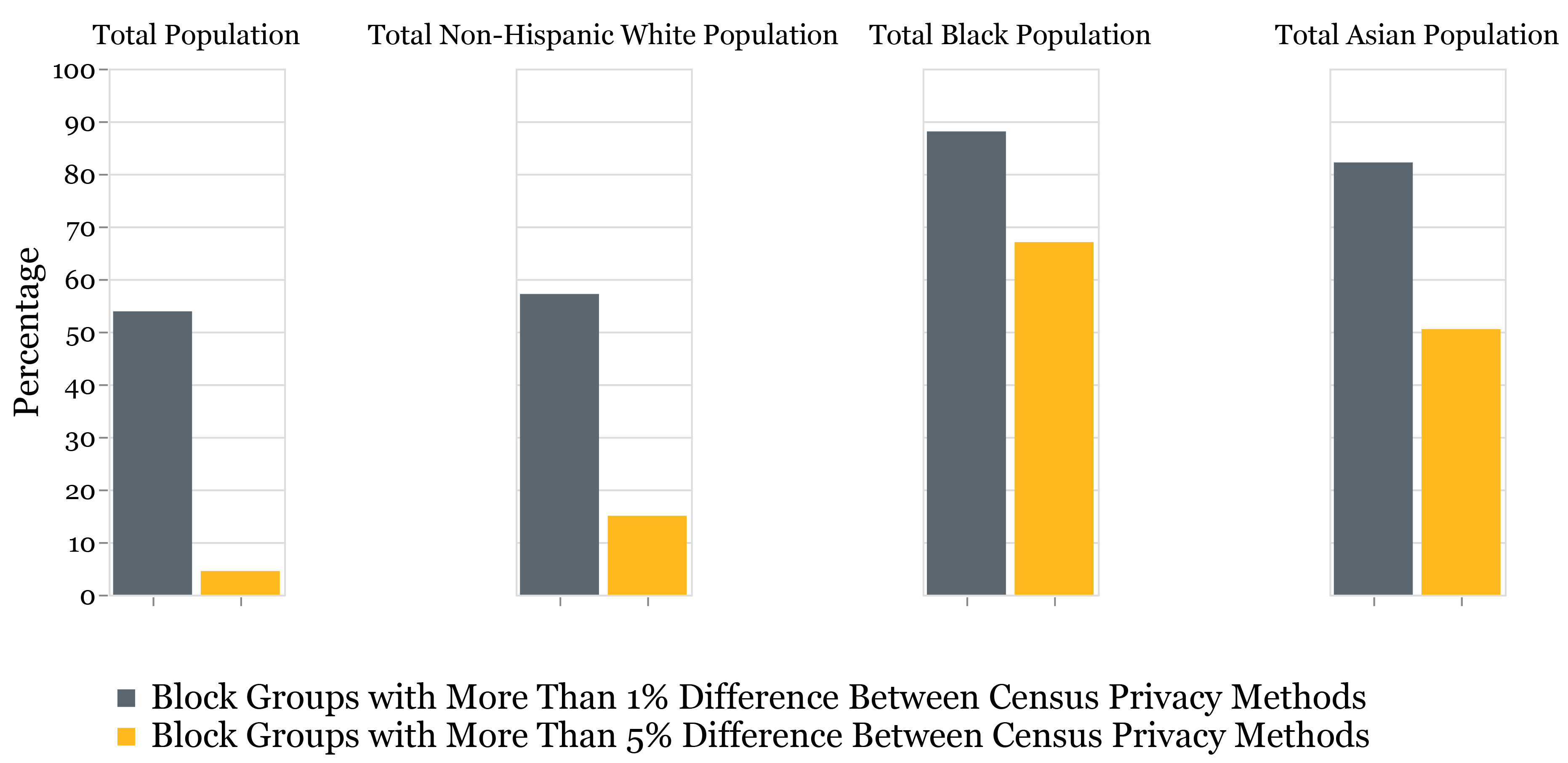 Source: Terner Center analysis of IPUMS NHGIS Census Data
Note: > 1% different also contains >5% different.
The problem is largest in block groups with smaller numbers of a particular demographic group. As figure 2 indicates, at small population sizes (especially with a population below 150) within the block group, there is a worrying difference between the two methods. Only when the group size within the block group increases past 350 and the difference between the methods drop below 2% do we feel comfortable with our results. This difference is especially troubling given that, in the 22,694 block groups in California that have a nonzero Black population, only 1,551 (~7%) have a Black population over 350. For a large swath of the state, we will not really be able to say whether or not declines (or gains) are meaningful changes.
Figure 2: Average Percentage Difference in California 2010 Black Population Between Census Privacy Methods by Block Group Subpopulation Size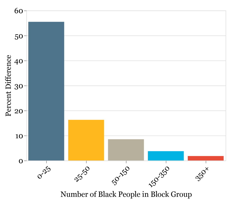 Source: Terner Center analysis of IPUMS NHGIS Census Data
The Census data remains a critical (and in many cases the only publicly available) source of information on our population, communities, and built environment. As the field incorporates the data into research, policy analysis, and policy making decisions, these new measures warrant careful consideration and engagement. At the Terner Center, we will continue to follow updates from the Census closely and take extra care in how we discuss evaluating demographic subcohort populations and smaller geographies in our research using the 2020 data.
To examine the results, you can access the code that created the charts and analysis in this blog post here and the IPUMS data for geographies other than block groups here.
Endnotes
- For example, the Census Bureau has developed a “blended base” for the 2021 American Community Survey (ACS) vintages, released the 2020 1-year ACS with experimental weights, and pushed back the release of the 2020 5-year ACS estimates from December 2021 to March 2022.
- Read the details of the Census’ differentially private “TopDown” algorithm from Abowd et al here. To simplify some very complicated math, an input (epsilon) controls the spread of a Laplace distribution wherein the random noise is added to the counts from which the data is drawn. As the noise is drawn at random from a distribution with a mean of zero, the aggregate estimates should be very close to the population aggregates, while making the user of the data unsure about the veracity of any specific data point. As you would expect, a wider distribution gives you more noise (meaning hypothetically more privacy protection and higher variance). The Census ultimately chose an epsilon of 19.61, which is reflected in the June 8th, 2021 vintage of data comparisons in the IPUMS data discussed in this article. As it is 1/ε that controls the spread of the distribution, the higher the epsilon, the lower the variance in the published data.
- All data used in the analysis for this blog post from David Van Riper, Tracy Kugler, and Jonathan Schroeder. IPUMS NHGIS Privacy-Protected 2010 Census Demonstration Data, version 20210608 [Database]. Minneapolis, MN: IPUMS. 2020.
- In the 2000 and 2010 Census there was a “swapping algorithm” implemented as an alternative method to protect privacy. This method had much less of an effect on the underlying data than TopDown does. Under the prior method, if at a block level there was an individual unique on some trait, that person would be swapped into a nearby block where that trait was shared by multiple others. This swapping aimed to protect individuals while not actually changing aggregate figures.
- Additionally, the number of occupied group quarters by major type (7 levels) in each block. These are referred to as the “invariants.”
- As well as for Places and Minor Civil Divisions with minimum total populations between 350 and 399.
- “Assessing the Reliability and Variability of the TopDown Algorithm for Redistricting Data” U.S. Census, June 03, 2021, https://www.census.gov/programs-surveys/decennial-census/decade/2020/planning-management/process/disclosure-avoidance/2020-das-updates/2021-06-03.html.
Share This Post:
Related Articles
Student Capstone Projects
As part of our commitment to the education and professional development of UC Berkeley students, the Terner Center highlights exceptional…
Lessons from California’s Statewide Efforts to Affirmatively Further Fair Housing
To counter the impacts of decades of discriminatory housing policies and worsening racial segregation, the State of California established a number of Affirmatively Furthering Fair Housing (AFFH) strategies. Designed to foster racially and economically inclusive, opportunity-rich communities, these efforts were intended to facilitate effective local fair housing planning and enacting statewide policies to promote integrated communities. A new Terner Center policy brief highlights key AFFH strategies, noting areas of progress and where additional efforts are needed. It examines California’s successes and challenges since 2016, offering recommendations for other states working toward fair housing goals.

Addressing the Housing Needs of Low-Income Households in the Bay Area: The Importance of Public Funding
This policy brief explores how public funding can address the San Francisco Bay Area's housing affordability crisis by increasing the…

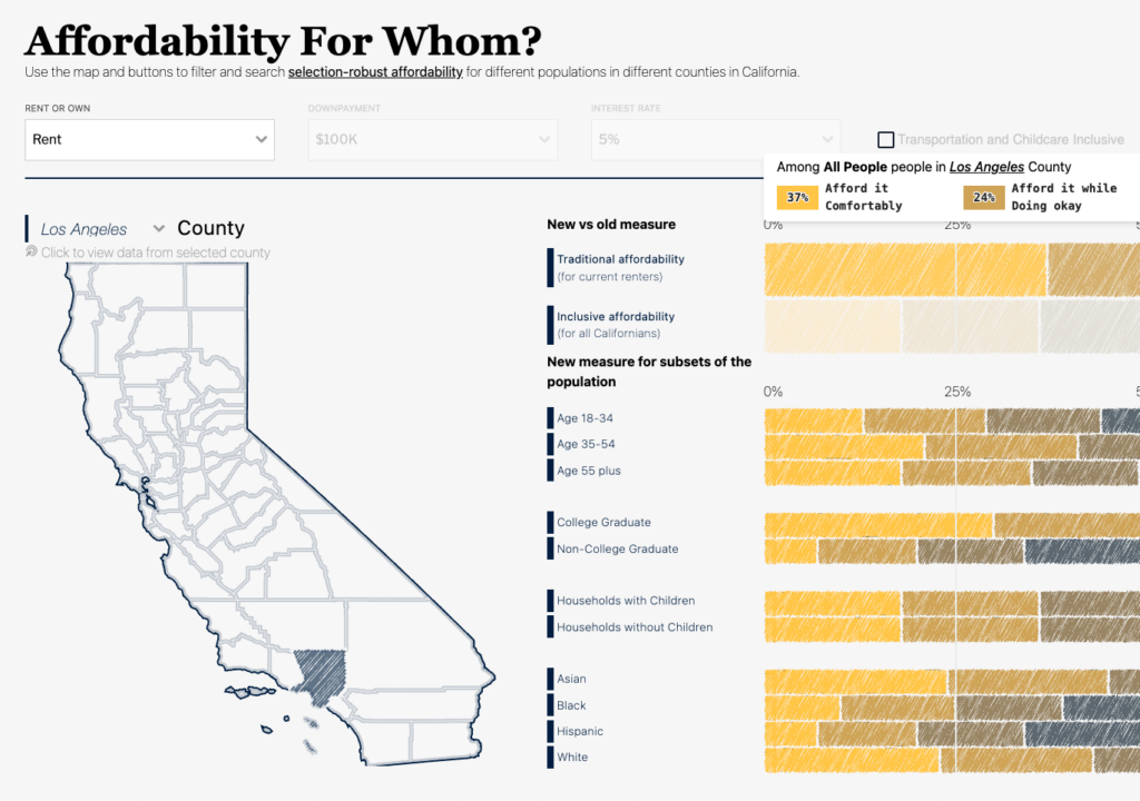
Affordability for Whom? Introducing an Inclusive Affordability Measure
This paper presents a new approach to measuring housing affordability—one that seeks to provide a better indicator of what counties…